Identify autophagy-positive cells¶

This notebook demonstrates how to train a machine learning model to distinguish between autophagy-positive and autophagy-negative cells using pre-calculated image features.

We define two classes based on autophagy induction in wild-type (WT) cells:

Class 0: Unstimulated WT cells
Class 1: 14h Torin-1 stimulated WT cells

After training and evaluating our model, we want to compare cells without a functional EI24 gene (EI24KO cells) to WT cells.

import numpy as np
import matplotlib.pyplot as plt
import seaborn as sns

import lamindb as ln
from anndata import concat

import scportrait
from sklearn.model_selection import train_test_split
from sklearn.ensemble import RandomForestClassifier
from sklearn.metrics import confusion_matrix, roc_curve, auc

ln.track()

Prepare ML model and data¶

def get_cells(dataframe):
    """Extract and concatenate single-cell data for cells specified in the input dataframe."""
    sc_data_list = []

    for uid in dataframe.dataset.unique():
        # Get cells for this dataset
        selected_cells = dataframe[dataframe.dataset == uid].copy()

        # Load single-cell data
        artifact_path = ln.Artifact.using("scportrait/examples").get(uid).cache()
        dataset = scportrait.io.read_h5sc(artifact_path)

        # Filter to selected cells
        dataset = dataset[
            dataset.obs.scportrait_cell_id.isin(
                selected_cells.scportrait_cell_id.values
            )
        ].copy()

        # Add prediction scores
        dataset.obs["score"] = selected_cells.prob_class1.values
        sc_data_list.append(dataset)

    sc_data = concat(sc_data_list, uns_merge="first", index_unique="-")
    sc_data.obs.reset_index(inplace=True, drop=True)
    sc_data.obs.index = sc_data.obs.index.values.astype(str)

    return sc_data

# Define RandomForest parameters
param_definitions = [
    ("random_state", "int"),
    ("n_estimators", "int"),
    ("max_depth", "int"),
    ("min_samples_split", "int"),
    ("min_samples_leaf", "int"),
    ("max_features", "str"),
    ("criterion", "str"),
    ("bootstrap", "bool"),
]

# Create parameter objects
for name, dtype in param_definitions:
    ln.Param(name=name, dtype=dtype).save()

rfc_params = {
    "random_state": 42,
    "n_estimators": 100,
    "max_depth": 10,
    "min_samples_split": 2,
    "min_samples_leaf": 1,
    "max_features": "sqrt",
    "criterion": "gini",
    "bootstrap": True,
}

ln.track(params=rfc_params)

study = ln.ULabel.using("scportrait/examples").get(name="autophagy imaging")

sc_datasets = (
    ln.Artifact.using("scportrait/examples")
    .filter(ulabels=study, is_latest=True)
    .filter(ulabels__name="scportrait single-cell images")
)

featurized_datasets = (
    ln.Artifact.using("scportrait/examples")
    .filter(ulabels=study, is_latest=True)
    .filter(description="featurized single-cell images")
)

class_lookup = {0: "untreated", 1: "14h Torin-1"}
label_lookup = {v: k for k, v in class_lookup.items()}

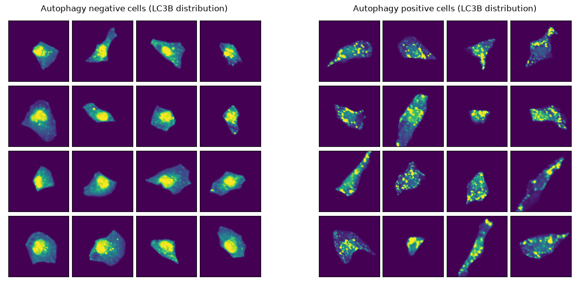
Let’s examine example images from both classes. As we can see, the cells look very distinct to one another. Hopefully our ML model will be able to separate them as well.

# Load example images for positive and negative autophagy
wt_cells = sc_datasets.filter(ulabels__name="WT")

autophagy_positive = scportrait.io.read_h5sc(
    wt_cells.filter(ulabels__name="14h Torin-1")[0].cache()
)
autophagy_negative = scportrait.io.read_h5sc(
    wt_cells.filter(ulabels__name="untreated")[0].cache()
)

# Plot negative and positive autophagy examples
channel_of_interest = 4  # LC3B channel: key autophagosome marker
num_rows, num_cols = 4, 4
n_cells = num_rows * num_cols

fig, axes = plt.subplots(1, 2, figsize=(15, 7))
examples = [
    (autophagy_negative, "Autophagy negative cells (LC3B distribution)", 0),
    (autophagy_positive, "Autophagy positive cells (LC3B distribution)", 1),
]

for data, title, ax_idx in examples:
    scportrait.pl.cell_grid_single_channel(
        data,
        select_channel=channel_of_interest,
        ax=axes[ax_idx],
        title=title,
        show_fig=False,
    )

Train ML model¶

We load the featurized datasets for both WT and EI24KO cells, then train a Random Forest model to distinguish between autophagy-positive and autophagy-negative states.

wt_cells_afs = (
    featurized_datasets.filter(ulabels__name="WT", is_latest=True).distinct().one()
)
features_wt = wt_cells_afs.load()

ko_cells_afs = (
    featurized_datasets.filter(ulabels__name="EI24KO", is_latest=True).distinct().one()
)
features_ko = ko_cells_afs.load()

# Split data
data_train, data_test = train_test_split(features_wt, test_size=0.4, random_state=42)

# Remove metadata and mCherry features, we will not use them for training
columns_to_drop = ["dataset", "scportrait_cell_id"] + [
    col for col in data_train.columns if "mCherry" in col
]

data_train_clean = data_train.drop(columns=columns_to_drop)
data_test_clean = data_test.drop(columns=columns_to_drop)

# Separate features and target variables
X_train = data_train_clean.drop("class", axis=1)
y_train = data_train_clean["class"]
X_test = data_test_clean.drop("class", axis=1)
y_test = data_test_clean["class"]

# Train model
clf = RandomForestClassifier(**rfc_params)
clf.fit(X_train, y_train)

# Make predictions
y_pred = clf.predict(X_test)
y_scores = clf.predict_proba(X_test)

data_test["predicted_class"] = y_pred
data_test["prob_class1"] = y_scores[:, 1]

We evaluate model performance using confusion matrices and ROC curves.

# Compute confusion matrix and ROC curve
cm = confusion_matrix(y_test, y_pred)
cm_normalized = cm.astype("float") / cm.sum(axis=1)[:, np.newaxis]
fpr, tpr, _ = roc_curve(y_test, y_scores[:, 1])
roc_auc = auc(fpr, tpr)

# Get class labels for display
class_labels = [class_lookup[label] for label in np.unique(y_test)]

fig, (ax_roc, ax_cm) = plt.subplots(1, 2, figsize=(12, 4))

# ROC
ax_roc.plot(fpr, tpr, color="blue", lw=2, label=f"ROC curve (AUC = {roc_auc:.2f})")
ax_roc.plot([0, 1], [0, 1], color="gray", linestyle="--")
ax_roc.set_xlim([0.0, 1.0])
ax_roc.set_ylim([0.0, 1.0])
ax_roc.set_xlabel("False Positive Rate")
ax_roc.set_ylabel("True Positive Rate")
ax_roc.set_title("ROC Curve")
ax_roc.legend(loc="lower right", frameon=False)

# Confusion matrix
sns.heatmap(
    cm_normalized,
    annot=True,
    fmt=".2f",
    cmap="Blues",
    xticklabels=class_labels,
    yticklabels=class_labels,
    ax=ax_cm,
    cbar=False,
)
ax_cm.set_xlabel("Predicted Label")
ax_cm.set_ylabel("True Label")
ax_cm.set_title("Confusion Matrix [% of true label]")

fig.tight_layout()

_images/96cabaedbdef08c425de630c0261894a753302655e6cd21c62f1475a515e201d.png

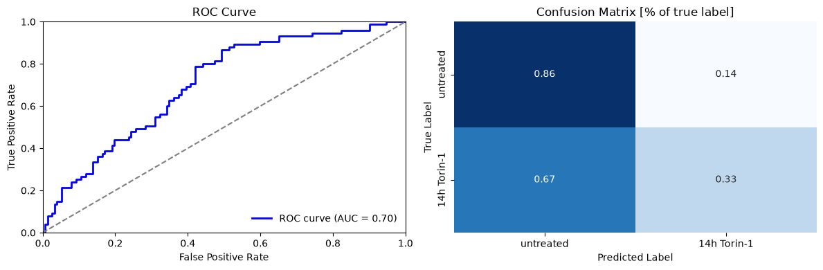
Despite being trained on a small dataset, our model performs reasonably well with an AUC of 0.7. The confusion matrix reveals that the classifier performs well at identifying autophagy-negative cells (86% accuracy) but struggles with autophagy-positive cells (less than 50% accuracy).

Let’s visualize example cells from each class to understand what patterns the model might be detecting.

# Visualize example cells from each prediction category
channel_of_interest = 4  # LC3B channel: key autophagosome marker
n_cells = 9

# Annotate dataset with prediction categories
data_test["TP"] = (data_test["class"] == 1) & (data_test["predicted_class"] == 1)
data_test["TN"] = (data_test["class"] == 0) & (data_test["predicted_class"] == 0)
data_test["FP"] = (data_test["class"] == 0) & (data_test["predicted_class"] == 1)
data_test["FN"] = (data_test["class"] == 1) & (data_test["predicted_class"] == 0)

# Get example cells for each category
cells_TP = (
    data_test[data_test.TP].sort_values("prob_class1", ascending=False).head(n_cells)
)
cells_TN = (
    data_test[data_test.TN].sort_values("prob_class1", ascending=False).tail(n_cells)
)
cells_FN = (
    data_test[data_test.FN].sort_values("prob_class1", ascending=False).tail(n_cells)
)
cells_FP = (
    data_test[data_test.FP].sort_values("prob_class1", ascending=False).head(n_cells)
)

cell_sets = {
    "TP": get_cells(cells_TP),
    "TN": get_cells(cells_TN),
    "FN": get_cells(cells_FN),
    "FP": get_cells(cells_FP),
}

fig, axes = plt.subplots(2, 2, figsize=(13, 13))
axes = axes.flatten()

for idx, (category, cells) in enumerate(cell_sets.items()):
    scportrait.pl.cell_grid_single_channel(
        cells,
        cell_ids=cells.obs.scportrait_cell_id,
        cell_labels=cells.obs.score.round(2).values,
        select_channel=channel_of_interest,
        ax=axes[idx],
        title=f"{category} with Prob(stimulated)",
        show_fig=False,
    )

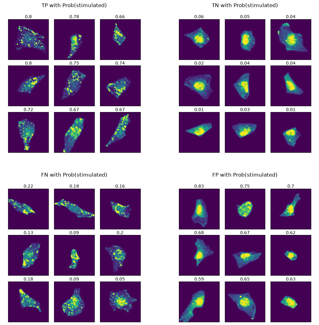
Analyzing model predictions

False Positives (FPs) - cells predicted as stimulated but actually unstimulated. We observe two distinct cell types:

Very small cells with no visible autophagosomes - likely genuine model errors
Larger cells with clear autophagosomes - these resemble TP cells more than TNs

The second type suggests our model may have discovered mislabeled data rather than making mistakes: cells can undergo spontaneous autophagy without Torin-1 treatment due to nutrient scarcity. Since our class labelling is based on cells having not been treated with Torin-1, we would be annotating these cells incorrectly.

False Negatives (FNs) - cells predicted as unstimulated but actually stimulated. These cells appear homogeneous and similar to TP cells, indicating model classification errors.

Before applying this model in a biological context, we should consider:

Expand training data to improve model robustness
Perform a pre-screening of our training data to ensure we remove any incorrectly labelled cells
Engineer better features that capture the biological processes of interest

For comparison, the original study achieved much higher accuracy using deep learning approaches on this same dataset.

Investigate the EI24 KO cells¶

Now let’s take a look at the EI24-deficient cells. EI24 deficiency is expected to disrupt autophagy induction, preventing normal responses to stimulation.

# Prepare KO data using same preprocessing as training data
columns_to_drop = ["dataset", "scportrait_cell_id"] + [
    col for col in features_ko.columns if "mCherry" in col
]
data_ko_clean = features_ko.drop(columns=columns_to_drop)

X_ko = data_ko_clean.drop("class", axis=1)
y_ko_true = data_ko_clean["class"]

# Make predictions on KO data
predictions_ko = clf.predict(X_ko)

# Compute and plot confusion matrix for KO cells
cm = confusion_matrix(y_ko_true, predictions_ko)
cm_normalized = cm.astype("float") / cm.sum(axis=1)[:, np.newaxis]

# Get class labels
class_labels = [class_lookup[label] for label in np.unique(y_ko_true)]

fig, ax = plt.subplots(1, 1, figsize=(4, 2))

sns.heatmap(
    cm_normalized,
    annot=True,
    fmt=".2f",
    cmap="Blues",
    xticklabels=class_labels,
    yticklabels=class_labels,
    ax=ax,
    cbar=False,
)
ax.set_xlabel("Predicted Label")
ax.set_ylabel("True Label")
ax.set_title("Confusion matrix [% of true label]")
fig.tight_layout()

_images/d7d45408e2f751eff63632210296a623256bd03eb4d6a593367cefd42df42f2e.png

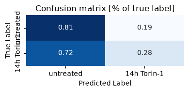
Interestingly, our model classifies a high percentage of stimulated EI24-KO cells as being unstimulated. Lets take a look at the images again.

# Compare WT and EI24KO cells
channel_of_interest = 4  # LC3B channel: key autophagosome marker

# Load EI24KO datasets
EI24_KO_unstimulated = scportrait.io.read_h5sc(
    sc_datasets.filter(ulabels__name="EI24KO")
    .filter(ulabels__name="untreated")[0]
    .cache()
)

EI24_KO_stimulated = scportrait.io.read_h5sc(
    sc_datasets.filter(ulabels__name="EI24KO")
    .filter(ulabels__name="14h Torin-1")[0]
    .cache()
)

fig, axes = plt.subplots(2, 2, figsize=(12, 12))

plot_data = [
    (autophagy_negative, "WT autophagy negative cells", (0, 0)),
    (autophagy_positive, "WT autophagy positive cells", (0, 1)),
    (EI24_KO_unstimulated, "EI24KO unstimulated cells", (1, 0)),
    (EI24_KO_stimulated, "EI24KO stimulated cells", (1, 1)),
]

for data, title, (row, col) in plot_data:
    scportrait.pl.cell_grid_single_channel(
        data,
        select_channel=channel_of_interest,
        ax=axes[row, col],
        title=title,
        show_fig=False,
    )

fig.tight_layout()

→ mapped: Artifact(uid='9KvNUZng67uxy4G90000')

→ mapped: Artifact(uid='wTSbpxi4KDY0FQql0000')

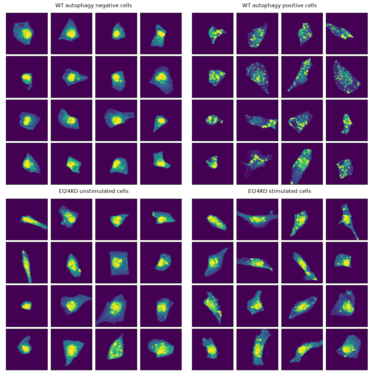
_images/fe4f05b02fcdf43980ef89a5e648c78793a6a858da4ad4e2f96dfd6b9a925804.png

The EI24 KO cells show fewer LC3 puncta and appear defective in autophagosome formation. Even after Torin-1 stimulation, EI24 KO cells look comparable to unstimulated cells.

This suggests our model correctly identifies the biological effect of EI24 deficiency - impaired autophagy induction even under stimulating conditions.

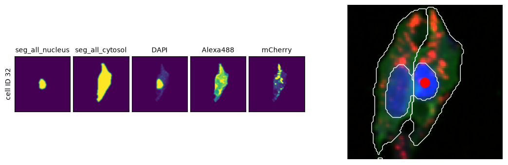
Visualize cells in their spatial context¶

As image analysis advances, obtaining the full context of a small section of the original image is often essential.

# Select a random cell from the WT dataset
cell = features_wt.sample(1, random_state=42)
dataset = cell["dataset"].values[0]
cell_id = cell["scportrait_cell_id"].values[0]

# Get SpatialData object and single-cell image dataset
sdata = (
    ln.Artifact.using("scportrait/examples")
    .get(
        key=ln.Artifact.using("scportrait/examples")
        .get(dataset)
        .key.replace("single_cell_data.h5ad", "spatialdata.zarr")
    )
    .load()
)
single_cell_images = scportrait.io.read_h5sc(ln.Artifact.get(dataset).cache())

# Get cell location coordinates
x, y = sdata["centers_seg_all_nucleus"].compute().loc[cell_id, :]

# Create comparison plot: single-cell view vs. spatial context
fig, (ax_cell, ax_spatial) = plt.subplots(1, 2, figsize=(12, 3.5))

# Plot single-cell images
scportrait.pl.cell_grid_multi_channel(
    single_cell_images, cell_ids=cell_id, ax=ax_cell, show_fig=False
)

# Plot spatial context with cell location highlighted
sdata_cropped = scportrait.tl.sdata.pp.get_bounding_box_sdata(
    sdata, center_x=x, center_y=y, max_width=100
)
scportrait.pl.plot_segmentation_mask(
    sdata_cropped,
    masks=["seg_all_nucleus", "seg_all_cytosol"],
    ax=ax_spatial,
    show_fig=False,
)
ax_spatial.scatter(x, y, color="red", s=200)

fig.tight_layout()

→ transferred: Artifact(uid='sF2ax2t7OJXkSId40003')

_images/6f12a67d305254a678629603582d5e279e07dc7b5bd272ff94fc7117610968d5.png

ln.finish()